Intro Project – Exploring Weather Trends

Overview

I have been provided the temperature database from the portal from where I have extracted the data related to global temperature and the temperature of New Delhi. I have analyzed and compared the temperature around the globle with New Delhi by selecting and extracting key data from the database.

Goals

1. Selecting city and country from the database “city_list”.
2. Extracting the City level data from the database “city_data” and export to CSV file.
3. Extracting the global temperature from the database “global_data” and export to CSV file.

Tools Used:

1. SQL: To extract the data from the database
2. Python: For calculating moving average and plotting line chart
3. ANACONDA – Jupyter Notebook: For writing python code, making observations and writing the project

Step 1: Extraction of data from the database

1. To check which countries and cities are available in the database.SELECT * FROM city_list WHERE Country='India' AND City='New Delhi';
2. To select data from the City database.SELECT avg_temp,year,city,country FROM city_data WHERE city='New Delhi';
3. I observed there is a column called avg_temp which is same in both city_data and global_data. I want to change the schema so I joined both the tables and changed the column names in both the databases.ALTER TABLE city_data RENAME COLUMN avg_temp to CAT; ALTER TABLE global_data RENAME COLUMN avg_temp to GAT;
4. I have joined the two tables using JOIN also called as INNER JOIN as avg_temp is same in both the tables.SELECT city_data.CAT, global_data.GAT, global_data.year FROM global_data JOIN city_data ON global_data.year = City_data.year WHERE city=’New Delhi’ Country=’India’;

Now, I have got an option to download a CSV file. I downloaded file as “results.csv”.

Step 2: Using Python for creating line charts

I have imported some python libraries here such as Numpy, Pandas (Matplotlib as well as Pyplot). I have written the code using Jupyter Notebook.

Observations:

1. The chart of the temperatures of New Delhi and Global Temperature shows that the difference between the average temperature of New Delhi and the World is very big.
2. The global data caused a slighty inclined result so I have plotted another graph for it which is the first graph.
3. The first graph shows the global temperature is increating constantly over the years by around 0.1 degree centigrade.
4. On the second graph I have observed that New Delhi has temperatures greater than the global average.
5. If I draw a line of best fit through the line of New Delhi, I can see a similar rise in temperature between New Delhi and the Global average over time. To verify this claim I used data.tail(10) to show me this trend continuing in the most recent years leading up to 2013.
6. New Delhi is a very hot city compared to most other cities in the world. From my research as a micro-study, New Delhi is surrounded by industrial factories and is nearby another city called Agra which also features large industrial facilities. Between them, they are two of the biggest industrial hubs in the world. I believe this may partly be the reason for the higher temperatures locally.

From my research as a macro-study, India itself lies nearer to the Equator so like most cities between the equator and the tropic of capricon or cancer it will have higher temperatures than the global average. Another reason for this is the area of these regions latitudally is very small compared to the rest of the globe so the temperatures fall as we move away from the equator. The Global Average Temperature is quite low compared to equatorial regions like New Delhi which can vary in temperature approximately between 8.4 to 9.6 degrees centigrade higher.

1. The temperature of the Globe is constantly rising from observing the second graph.

Considerations:

1. X-Axis: Years.
2. Y-Axis: Temperature(°C).
3. Different colors of lines for city and global average.
4. Use of Matplotlib library for visualization.
5. Applied Moving Average (MA) on city_data in order to get a relatively smooth line.
6. Defined functions for easier to understand coding.
7. Saved all of the code in .ipynb files (Jupyter Notebook) for later reference or revisions.

References:

1. Change Column Name: https://www.1keydata.com/sql/alter-table-rename-column.html
2. Joining the tables: http://www.dofactory.com/sql/join
3. Calculation command for Moving Average in Python: http://www.learndatasci.com/python-finance-part-3-moving-average-tradingstrategy/
4. Parameters for .rolling() https://pandas.pydata.org/pandas-docs/stable/generated/pandas.DataFrame.rolling.html

In [1]:

# Importing the important Libraries
import numpy as np
import pandas as pd # for loading data into the notebook
from matplotlib import pyplot as plt #for making line chart

In [2]:

# Importing the extracted Data Set
data = pd.read_csv( "results.csv" )

In [3]:

data

Out[3]:

	year	gat	cat
0	1796	8.27	25.03
1	1797	8.51	26.71
2	1798	8.67	24.29
3	1799	8.51	25.28
4	1800	8.48	25.21
5	1801	8.59	24.22
6	1802	8.58	25.63
7	1803	8.50	25.38
8	1804	8.84	25.68
9	1805	8.56	25.30
10	1806	8.43	25.22
11	1807	8.28	24.97
12	1808	7.63	NaN
13	1809	7.08	NaN
14	1810	6.92	NaN
15	1811	6.86	NaN
16	1812	7.05	NaN
17	1813	7.74	24.56
18	1814	7.59	23.73
19	1815	7.24	24.09
20	1816	6.94	23.70
21	1817	6.98	23.86
22	1818	7.83	24.37
23	1819	7.37	23.90
24	1820	7.62	24.12
25	1821	8.09	24.83
26	1822	8.19	24.93
27	1823	7.72	24.63
28	1824	8.55	25.30
29	1825	8.39	25.11
…	…	…	…
188	1984	8.69	25.56
189	1985	8.66	25.86
190	1986	8.83	25.31
191	1987	8.99	26.54
192	1988	9.20	26.11
193	1989	8.92	25.43
194	1990	9.23	25.54
195	1991	9.18	25.74
196	1992	8.84	25.52
197	1993	8.87	25.92
198	1994	9.04	25.87
199	1995	9.35	25.92
200	1996	9.04	25.55
201	1997	9.20	24.71
202	1998	9.52	25.77
203	1999	9.29	26.36
204	2000	9.20	26.05
205	2001	9.41	25.86
206	2002	9.57	26.63
207	2003	9.53	25.72
208	2004	9.32	26.24
209	2005	9.70	25.72
210	2006	9.53	26.37
211	2007	9.73	26.15
212	2008	9.43	25.68
213	2009	9.51	26.55
214	2010	9.70	26.52
215	2011	9.52	25.63
216	2012	9.51	25.89
217	2013	9.61	26.71

218 rows × 3 columns

This should define a function for the calculation of moving averages in order to get smooth graph. And data.info should help show the data more clearly.In [4]:

# function that calculates the MOVING AVERAGE
def moving_avg (mA_range, data_input):
    output = data_input.rolling(window = mA_range, on = "cat" ).mean().dropna()
    return output

In [5]:

# Function Calling with the range of Moving Average
mA_value = 150
chart_moving_avg = moving_avg(mA_value, data)

In [6]:

# Drawing the graph: Global Temperature
plt.plot(chart_moving_avg [ 'year' ], chart_moving_avg [ 'gat' ], label = 'Global' )
plt.legend()
plt.xlabel ( "Years" )
plt.ylabel ( "Temperature (°C)" )
plt.title ( "Global Average Temperature" )
plt.show ()

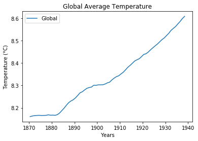
Above is the output. Next, I have analysed the global data separately in order to check and distinguish it from combined data of New Delhi and Global Average temperatures.

Now combined with New Delhi data:In [7]:

# Drawing the graph: New Delhi and Global Temperature
# Introducing this line in the previous code above the “global_data plot command”
plt.plot(chart_moving_avg ['year'], chart_moving_avg ['cat'], label = 'New Delhi')
plt.plot(chart_moving_avg ['year'], chart_moving_avg ['gat'], label = 'Global')
plt.legend()
plt.xlabel ( "Years" )
plt.ylabel ( "Temperature (°C)" )
plt.title ( "New Delhi and Global Temperature" )
plt.show ()

Above is the resulting graph. I have analysed my results further by adding:In [8]:

data.head (10)

Out[8]:

	year	gat	cat
0	1796	8.27	25.03
1	1797	8.51	26.71
2	1798	8.67	24.29
3	1799	8.51	25.28
4	1800	8.48	25.21
5	1801	8.59	24.22
6	1802	8.58	25.63
7	1803	8.50	25.38
8	1804	8.84	25.68
9	1805	8.56	25.30

In [9]:

data.tail (10)

Out[9]:

	year	gat	cat
208	2004	9.32	26.24
209	2005	9.70	25.72
210	2006	9.53	26.37
211	2007	9.73	26.15
212	2008	9.43	25.68
213	2009	9.51	26.55
214	2010	9.70	26.52
215	2011	9.52	25.63
216	2012	9.51	25.89
217	2013	9.61	26.71

In [ ]: