Project 4 – Communicate Data Findings

Table of Contents

• Introduction of the topic and dataset
• Dataset Investigation and preliminary wrangling
• Further Data Wrangling
• Univariate Exploration and Analysis
• Bivariate Exploration and Analysis
• Multivariate Exploration and Analysis
• Conclusions and Answers

Introduction of the topic and dataset

Introduction to PISA

What Is PISA?

The Program for International Student Assessment (PISA) is a system of international assessments that allows countries to compare outcomes of learning as students near the end of compulsory schooling. PISA core assessments measure the performance of 15-year-old students in mathematics, science, and reading literacy every 3 years. Coordinated by the Organization for Economic Cooperation and Development (OECD), PISA was first implemented in 2000 in 32 countries. It has since grown to 65 education systems in 2012.

Project Aims

Project: Data Exploration of the performance of globally-selected 15/16-year-old students in Mathematics, Reading and Science Literacy, based on the results of the PISA 2012 test

What PISA Measures

PISA’s goal is to assess students’ preparation for the challenges of life as young adults. PISA assesses the application of knowledge in mathematics, science, and reading literacy to problems within a reallife context (OECD 1999). PISA does not focus explicitly on curricular outcomes and uses the term “literacy” in each subject area to indicate its broad focus on the application of knowledge and skills. For example, when assessing mathematics, PISA examines how well 15-year-old students can understand, use, and reflect on mathematics for a variety of real-life problems and settings that they may not encounter in the classroom. Scores on the PISA scales represent skill levels along a continuum of literacy skills.

Each PISA data collection cycle assesses one of the three core subject areas in depth (considered the major subject area), although all three core subjects are assessed in each cycle (the other two subjects are considered minor subject areas for that assessment year). Assessing all three subjects every 3 years allows countries to have a consistent source of achievement data in each of the three subjects, while rotating one area as the primary focus over the years. Mathematics was the major subject area in 2012, as it was in 2003, since each subject is a major subject area once every three cycles. In 2012, mathematics, science, and reading literacy were assessed primarily through a paper-and-pencil assessment, and problem solving was administered via a computer-based assessment. In addition to these core assessments, education systems could participate in optional paper-based financial literacy and computer-based mathematics and reading assessments. The United States participated in these optional assessments. Visit www.nces.ed.gov/surveys/pisa for more information on the PISA assessments, including information on how the assessments were designed and examples of PISA questions.

Ref.: NCES 2014-024, U.S. Department of Education

Introduction to the PISA 2012 dataset

PISA is a survey of students’ skills and knowledge as they approach the end of compulsory education. It is not a conventional school test. Rather than examining how well students have learned the school curriculum, it looks at how well prepared they are for life beyond school.

Around 510,000 students in 65 economies took part in the PISA 2012 assessment of reading, mathematics and science representing about 28 million 15-year-olds globally. Of those economies, 44 took part in an assessment of creative problem solving and 18 in an assessment of financial literacy.In [1]:

# import all packages and set plots to be embedded inline
import numpy as np
import pandas as pd
import matplotlib.pyplot as plt
import seaborn as sb

%matplotlib inline

sb.set()

# We are interested in exploring the formatting of all columns (variables), hence we will display all of them
pd.set_option('display.max_rows', 636)
pd.set_option('display.max_columns', 636)

In [2]:

df = pd.read_csv('pisa2012.csv', encoding='latin-1', low_memory = False)

In [3]:

df.head(3)

Out[3]:

	Unnamed: 0	CNT	SUBNATIO	STRATUM	OECD	NC	SCHOOLID	STIDSTD	ST01Q01	ST02Q01	ST03Q01	ST03Q02	ST04Q01	ST05Q01	ST06Q01	ST07Q01	ST07Q02	ST07Q03	ST08Q01	ST09Q01	ST115Q01	ST11Q01	ST11Q02	ST11Q03	ST11Q04	ST11Q05	ST11Q06	ST13Q01	ST14Q01	ST14Q02	ST14Q03	ST14Q04	ST15Q01	ST17Q01	ST18Q01	ST18Q02	ST18Q03	ST18Q04	ST19Q01	ST20Q01	ST20Q02	ST20Q03	ST21Q01	ST25Q01	ST26Q01	ST26Q02	ST26Q03	ST26Q04	ST26Q05	ST26Q06	ST26Q07	ST26Q08	ST26Q09	ST26Q10	ST26Q11	ST26Q12	ST26Q13	ST26Q14	ST26Q15	ST26Q16	ST26Q17	ST27Q01	ST27Q02	ST27Q03	ST27Q04	ST27Q05	ST28Q01	ST29Q01	ST29Q02	ST29Q03	ST29Q04	ST29Q05	ST29Q06	ST29Q07	ST29Q08	ST35Q01	ST35Q02	ST35Q03	ST35Q04	ST35Q05	ST35Q06	ST37Q01	ST37Q02	ST37Q03	ST37Q04	ST37Q05	ST37Q06	ST37Q07	ST37Q08	ST42Q01	ST42Q02	ST42Q03	ST42Q04	ST42Q05	ST42Q06	ST42Q07	ST42Q08	ST42Q09	ST42Q10	ST43Q01	ST43Q02	ST43Q03	ST43Q04	ST43Q05	ST43Q06	ST44Q01	ST44Q03	ST44Q04	ST44Q05	ST44Q07	ST44Q08	ST46Q01	ST46Q02	ST46Q03	ST46Q04	ST46Q05	ST46Q06	ST46Q07	ST46Q08	ST46Q09	ST48Q01	ST48Q02	ST48Q03	ST48Q04	ST48Q05	ST49Q01	ST49Q02	ST49Q03	ST49Q04	ST49Q05	ST49Q06	ST49Q07	ST49Q09	ST53Q01	ST53Q02	ST53Q03	ST53Q04	ST55Q01	ST55Q02	ST55Q03	ST55Q04	ST57Q01	ST57Q02	ST57Q03	ST57Q04	ST57Q05	ST57Q06	ST61Q01	ST61Q02	ST61Q03	ST61Q04	ST61Q05	ST61Q06	ST61Q07	ST61Q08	ST61Q09	ST62Q01	ST62Q02	ST62Q03	ST62Q04	ST62Q06	ST62Q07	ST62Q08	ST62Q09	ST62Q10	ST62Q11	ST62Q12	ST62Q13	ST62Q15	ST62Q16	ST62Q17	ST62Q19	ST69Q01	ST69Q02	ST69Q03	ST70Q01	ST70Q02	ST70Q03	ST71Q01	ST72Q01	ST73Q01	ST73Q02	ST74Q01	ST74Q02	ST75Q01	ST75Q02	ST76Q01	ST76Q02	ST77Q01	ST77Q02	ST77Q04	ST77Q05	ST77Q06	ST79Q01	ST79Q02	ST79Q03	ST79Q04	ST79Q05	ST79Q06	ST79Q07	ST79Q08	ST79Q10	ST79Q11	ST79Q12	ST79Q15	ST79Q17	ST80Q01	ST80Q04	ST80Q05	ST80Q06	ST80Q07	ST80Q08	ST80Q09	ST80Q10	ST80Q11	ST81Q01	ST81Q02	ST81Q03	ST81Q04	ST81Q05	ST82Q01	ST82Q02	ST82Q03	ST83Q01	ST83Q02	ST83Q03	ST83Q04	ST84Q01	ST84Q02	ST84Q03	ST85Q01	ST85Q02	ST85Q03	ST85Q04	ST86Q01	ST86Q02	ST86Q03	ST86Q04	ST86Q05	ST87Q01	ST87Q02	ST87Q03	ST87Q04	ST87Q05	ST87Q06	ST87Q07	ST87Q08	ST87Q09	ST88Q01	ST88Q02	ST88Q03	ST88Q04	ST89Q02	ST89Q03	ST89Q04	ST89Q05	ST91Q01	ST91Q02	ST91Q03	ST91Q04	ST91Q05	ST91Q06	ST93Q01	ST93Q03	ST93Q04	ST93Q06	ST93Q07	ST94Q05	ST94Q06	ST94Q09	ST94Q10	ST94Q14	ST96Q01	ST96Q02	ST96Q03	ST96Q05	ST101Q01	ST101Q02	ST101Q03	ST101Q05	ST104Q01	ST104Q04	ST104Q05	ST104Q06	IC01Q01	IC01Q02	IC01Q03	IC01Q04	IC01Q05	IC01Q06	IC01Q07	IC01Q08	IC01Q09	IC01Q10	IC01Q11	IC02Q01	IC02Q02	IC02Q03	IC02Q04	IC02Q05	IC02Q06	IC02Q07	IC03Q01	IC04Q01	IC05Q01	IC06Q01	IC07Q01	IC08Q01	IC08Q02	IC08Q03	IC08Q04	IC08Q05	IC08Q06	IC08Q07	IC08Q08	IC08Q09	IC08Q11	IC09Q01	IC09Q02	IC09Q03	IC09Q04	IC09Q05	IC09Q06	IC09Q07	IC10Q01	IC10Q02	IC10Q03	IC10Q04	IC10Q05	IC10Q06	IC10Q07	IC10Q08	IC10Q09	IC11Q01	IC11Q02	IC11Q03	IC11Q04	IC11Q05	IC11Q06	IC11Q07	IC22Q01	IC22Q02	IC22Q04	IC22Q06	IC22Q07	IC22Q08	EC01Q01	EC02Q01	EC03Q01	EC03Q02	EC03Q03	EC03Q04	EC03Q05	EC03Q06	EC03Q07	EC03Q08	EC03Q09	EC03Q10	EC04Q01A	EC04Q01B	EC04Q01C	EC04Q02A	EC04Q02B	EC04Q02C	EC04Q03A	EC04Q03B	EC04Q03C	EC04Q04A	EC04Q04B	EC04Q04C	EC04Q05A	EC04Q05B	EC04Q05C	EC04Q06A	EC04Q06B	EC04Q06C	EC05Q01	EC06Q01	EC07Q01	EC07Q02	EC07Q03	EC07Q04	EC07Q05	EC08Q01	EC08Q02	EC08Q03	EC08Q04	EC09Q03	EC10Q01	EC11Q02	EC11Q03	EC12Q01	ST22Q01	ST23Q01	ST23Q02	ST23Q03	ST23Q04	ST23Q05	ST23Q06	ST23Q07	ST23Q08	ST24Q01	ST24Q02	ST24Q03	CLCUSE1	CLCUSE301	CLCUSE302	DEFFORT	QUESTID	BOOKID	EASY	AGE	GRADE	PROGN	ANXMAT	ATSCHL	ATTLNACT	BELONG	BFMJ2	BMMJ1	CLSMAN	COBN_F	COBN_M	COBN_S	COGACT	CULTDIST	CULTPOS	DISCLIMA	ENTUSE	ESCS	EXAPPLM	EXPUREM	FAILMAT	FAMCON	FAMCONC	FAMSTRUC	FISCED	HEDRES	HERITCUL	HISCED	HISEI	HOMEPOS	HOMSCH	HOSTCUL	ICTATTNEG	ICTATTPOS	ICTHOME	ICTRES	ICTSCH	IMMIG	INFOCAR	INFOJOB1	INFOJOB2	INSTMOT	INTMAT	ISCEDD	ISCEDL	ISCEDO	LANGCOMM	LANGN	LANGRPPD	LMINS	MATBEH	MATHEFF	MATINTFC	MATWKETH	MISCED	MMINS	MTSUP	OCOD1	OCOD2	OPENPS	OUTHOURS	PARED	PERSEV	REPEAT	SCMAT	SMINS	STUDREL	SUBNORM	TCHBEHFA	TCHBEHSO	TCHBEHTD	TEACHSUP	TESTLANG	TIMEINT	USEMATH	USESCH	WEALTH	ANCATSCHL	ANCATTLNACT	ANCBELONG	ANCCLSMAN	ANCCOGACT	ANCINSTMOT	ANCINTMAT	ANCMATWKETH	ANCMTSUP	ANCSCMAT	ANCSTUDREL	ANCSUBNORM	PV1MATH	PV2MATH	PV3MATH	PV4MATH	PV5MATH	PV1MACC	PV2MACC	PV3MACC	PV4MACC	PV5MACC	PV1MACQ	PV2MACQ	PV3MACQ	PV4MACQ	PV5MACQ	PV1MACS	PV2MACS	PV3MACS	PV4MACS	PV5MACS	PV1MACU	PV2MACU	PV3MACU	PV4MACU	PV5MACU	PV1MAPE	PV2MAPE	PV3MAPE	PV4MAPE	PV5MAPE	PV1MAPF	PV2MAPF	PV3MAPF	PV4MAPF	PV5MAPF	PV1MAPI	PV2MAPI	PV3MAPI	PV4MAPI	PV5MAPI	PV1READ	PV2READ	PV3READ	PV4READ	PV5READ	PV1SCIE	PV2SCIE	PV3SCIE	PV4SCIE	PV5SCIE	W_FSTUWT	W_FSTR1	W_FSTR2	W_FSTR3	W_FSTR4	W_FSTR5	W_FSTR6	W_FSTR7	W_FSTR8	W_FSTR9	W_FSTR10	W_FSTR11	W_FSTR12	W_FSTR13	W_FSTR14	W_FSTR15	W_FSTR16	W_FSTR17	W_FSTR18	W_FSTR19	W_FSTR20	W_FSTR21	W_FSTR22	W_FSTR23	W_FSTR24	W_FSTR25	W_FSTR26	W_FSTR27	W_FSTR28	W_FSTR29	W_FSTR30	W_FSTR31	W_FSTR32	W_FSTR33	W_FSTR34	W_FSTR35	W_FSTR36	W_FSTR37	W_FSTR38	W_FSTR39	W_FSTR40	W_FSTR41	W_FSTR42	W_FSTR43	W_FSTR44	W_FSTR45	W_FSTR46	W_FSTR47	W_FSTR48	W_FSTR49	W_FSTR50	W_FSTR51	W_FSTR52	W_FSTR53	W_FSTR54	W_FSTR55	W_FSTR56	W_FSTR57	W_FSTR58	W_FSTR59	W_FSTR60	W_FSTR61	W_FSTR62	W_FSTR63	W_FSTR64	W_FSTR65	W_FSTR66	W_FSTR67	W_FSTR68	W_FSTR69	W_FSTR70	W_FSTR71	W_FSTR72	W_FSTR73	W_FSTR74	W_FSTR75	W_FSTR76	W_FSTR77	W_FSTR78	W_FSTR79	W_FSTR80	WVARSTRR	VAR_UNIT	SENWGT_STU	VER_STU
0	1	Albania	80000	ALB0006	Non-OECD	Albania	1	1	10	1.0	2	1996	Female	No	6.0	No, never	No, never	No, never	None	None	1.0	Yes	Yes	Yes	Yes	NaN	NaN	<ISCED level 3A>	No	No	No	No	Other (e.g. home duties, retired)	<ISCED level 3A>	NaN	NaN	NaN	NaN	Working part-time <for pay>	Country of test	Country of test	Country of test	NaN	Language of the test	Yes	No	Yes	No	No	No	No	Yes	No	Yes	No	Yes	No	Yes	8002	8001	8002	Two	One	None	None	None	0-10 books	Agree	Strongly agree	Agree	Agree	Agree	Agree	Agree	Strongly agree	Disagree	Agree	Disagree	Agree	Agree	Agree	Not at all confident	Not very confident	Confident	Confident	Confident	Not at all confident	Confident	Very confident	Agree	Disagree	Agree	Agree	Agree	Agree	Agree	Disagree	Disagree	Disagree	Agree	Disagree	Disagree	Agree	NaN	Disagree	Likely	Slightly likely	Likely	Likely	Likely	Very Likely	Agree	Agree	Agree	Agree	Agree	Agree	Agree	Agree	Agree	Courses after school Test Language	Major in college Science	Study harder Test Language	Maximum classes Science	Pursuing a career Math	Often	Sometimes	Sometimes	Sometimes	Sometimes	Never or rarely	Never or rarely	Never or rarely	NaN	NaN	NaN	NaN	NaN	NaN	NaN	NaN	NaN	NaN	NaN	NaN	NaN	NaN	NaN	NaN	NaN	NaN	NaN	NaN	NaN	NaN	NaN	NaN	NaN	NaN	NaN	NaN	NaN	NaN	NaN	NaN	NaN	NaN	NaN	NaN	NaN	NaN	NaN	NaN	NaN	NaN	NaN	NaN	NaN	NaN	NaN	NaN	NaN	NaN	NaN	NaN	NaN	NaN	NaN	Every Lesson	Every Lesson	Every Lesson	Every Lesson	Every Lesson	Never or Hardly Ever	Most Lessons	Never or Hardly Ever	Every Lesson	Most Lessons	Every Lesson	Every Lesson	Every Lesson	Never or Hardly Ever	Most Lessons	Every Lesson	Every Lesson	Every Lesson	Always or almost always	Sometimes	Never or rarely	Always or almost always	Always or almost always	Always or almost always	Always or almost always	Often	Often	Never or Hardly Ever	Never or Hardly Ever	Never or Hardly Ever	Never or Hardly Ever	Never or Hardly Ever	Strongly disagree	Strongly disagree	Strongly disagree	Strongly disagree	Agree	Agree	Agree	Strongly agree	Strongly agree	Disagree	Agree	Strongly disagree	Disagree	Agree	Agree	Strongly disagree	Agree	Agree	Disagree	Agree	Agree	Strongly disagree	Strongly agree	Strongly agree	Strongly disagree	Agree	Strongly disagree	Agree	Agree	Strongly agree	Strongly disagree	Strongly disagree	Agree	Strongly agree	Strongly agree	Strongly agree	Strongly agree	Strongly agree	Strongly agree	Strongly disagree	Disagree	Strongly disagree	Very much like me	Very much like me	Very much like me	Somewhat like me	Very much like me	Somewhat like me	Mostly like me	Mostly like me	Mostly like me	Somewhat like me	definitely do this	definitely do this	definitely do this	definitely do this	4.0	2.0	1.0	1.0	1.0	2.0	1.0	1.0	NaN	NaN	NaN	NaN	NaN	NaN	NaN	NaN	NaN	NaN	NaN	NaN	NaN	NaN	NaN	NaN	NaN	NaN	NaN	NaN	99	99	99	NaN	NaN	NaN	NaN	NaN	NaN	NaN	NaN	NaN	NaN	NaN	NaN	NaN	NaN	NaN	NaN	NaN	NaN	NaN	NaN	NaN	NaN	NaN	NaN	NaN	NaN	NaN	NaN	NaN	NaN	NaN	NaN	NaN	NaN	NaN	NaN	NaN	NaN	NaN	NaN	NaN	NaN	NaN	NaN	NaN	NaN	NaN	NaN	NaN	NaN	NaN	NaN	NaN	NaN	NaN	NaN	NaN	NaN	NaN	NaN	NaN	NaN	NaN	NaN	NaN	NaN	NaN	NaN	NaN	NaN	NaN	NaN	NaN	NaN	NaN	NaN	NaN	NaN	NaN	NaN	NaN	NaN	NaN	NaN	NaN	NaN	NaN	NaN	NaN	NaN	NaN	NaN	NaN	NaN	NaN	NaN	NaN	A Simple calculator	99	99	99	StQ Form B	booklet 7	Standard set of booklets	16.17	0.0	Albania: Upper secondary education	0.32	-2.31	0.5206	-1.18	76.49	79.74	-1.3771	Albania	Albania	Albania	0.6994	NaN	-0.48	1.85	NaN	NaN	NaN	NaN	0.6400	NaN	NaN	2.0	ISCED 3A, ISCED 4	-1.29	NaN	ISCED 3A, ISCED 4	NaN	-2.61	NaN	NaN	NaN	NaN	NaN	-3.16	NaN	Native	NaN	NaN	NaN	0.80	0.91	A	ISCED level 3	General	NaN	Albanian	NaN	NaN	0.6426	-0.77	-0.7332	0.2882	ISCED 3A, ISCED 4	NaN	-0.9508	Building architects	Primary school teachers	0.0521	NaN	12.0	-0.3407	Did not repeat a <grade>	0.41	NaN	-1.04	-0.0455	1.3625	0.9374	0.4297	1.68	Albanian	NaN	NaN	NaN	-2.92	-1.8636	-0.6779	-0.7351	-0.7808	-0.0219	-0.1562	0.0486	-0.2199	-0.5983	-0.0807	-0.5901	-0.3346	406.8469	376.4683	344.5319	321.1637	381.9209	325.8374	324.2795	279.8800	267.4170	312.5954	409.1837	388.1524	373.3525	389.7102	415.4152	351.5423	375.6894	341.4161	386.5945	426.3203	396.7207	334.4057	328.9531	339.8582	354.6580	324.2795	345.3108	381.1419	380.3630	346.8687	319.6059	345.3108	360.8895	390.4892	322.7216	290.7852	345.3108	326.6163	407.6258	367.1210	249.5762	254.3420	406.8496	175.7053	218.5981	341.7009	408.8400	348.2283	367.8105	392.9877	8.9096	13.1249	13.0829	4.5315	13.0829	13.9235	13.1249	13.1249	4.3389	4.3313	13.7954	4.5315	4.3313	13.7954	13.9235	4.3389	4.3313	4.5084	4.5084	13.7954	4.5315	13.1249	13.0829	4.5315	13.0829	13.9235	13.1249	13.1249	4.3389	4.3313	13.7954	4.5315	4.3313	13.7954	13.9235	4.3389	4.3313	4.5084	4.5084	13.7954	4.5315	4.5084	4.5315	13.0829	4.5315	4.3313	4.5084	4.5084	13.7954	13.9235	4.3389	13.0829	13.9235	4.3389	4.3313	13.7954	13.9235	13.1249	13.1249	4.3389	13.0829	4.5084	4.5315	13.0829	4.5315	4.3313	4.5084	4.5084	13.7954	13.9235	4.3389	13.0829	13.9235	4.3389	4.3313	13.7954	13.9235	13.1249	13.1249	4.3389	13.0829	19	1	0.2098	22NOV13
1	2	Albania	80000	ALB0006	Non-OECD	Albania	1	2	10	1.0	2	1996	Female	Yes, for more than one year	7.0	No, never	No, never	No, never	One or two times	None	1.0	Yes	Yes	NaN	Yes	NaN	NaN	<ISCED level 3A>	Yes	Yes	No	No	Working full-time <for pay>	<ISCED level 3A>	No	No	No	No	Working full-time <for pay>	Country of test	Country of test	Country of test	NaN	Language of the test	Yes	Yes	Yes	Yes	Yes	Yes	Yes	Yes	Yes	Yes	Yes	Yes	Yes	Yes	8001	8001	8002	Three or more	Three or more	Three or more	Two	Two	201-500 books	Disagree	Strongly agree	Disagree	Disagree	Agree	Agree	Disagree	Disagree	Strongly agree	Strongly agree	Disagree	Agree	Disagree	Agree	Confident	Very confident	Very confident	Confident	Very confident	Confident	Very confident	Not very confident	NaN	NaN	NaN	NaN	NaN	NaN	NaN	NaN	NaN	NaN	Strongly agree	Strongly agree	Strongly disagree	Disagree	Agree	Disagree	Likely	Slightly likely	Slightly likely	Very Likely	Slightly likely	Likely	Agree	Agree	Strongly agree	Strongly agree	Strongly agree	Agree	Agree	Disagree	Agree	Courses after school Math	Major in college Science	Study harder Math	Maximum classes Science	Pursuing a career Science	Sometimes	Often	Always or almost always	Sometimes	Always or almost always	Never or rarely	Never or rarely	Often	relating to known	Improve understanding	in my sleep	Repeat examples	I do not attend <out-of-school time lessons> i…	2 or more but less than 4 hours a week	2 or more but less than 4 hours a week	Less than 2 hours a week	NaN	NaN	6.0	0.0	0.0	2.0	Rarely	Rarely	Frequently	Sometimes	Frequently	Sometimes	Frequently	Never	Frequently	Know it well, understand the concept	Know it well, understand the concept	Heard of it once or twice	Know it well, understand the concept	Know it well, understand the concept	Know it well, understand the concept	Never heard of it	Know it well, understand the concept	Know it well, understand the concept	Never heard of it	Know it well, understand the concept	Heard of it once or twice	Know it well, understand the concept	Know it well, understand the concept	Never heard of it	Heard of it often	45.0	45.0	45.0	7.0	6.0	2.0	NaN	30.0	Frequently	Sometimes	Frequently	Frequently	Sometimes	Sometimes	Sometimes	Sometimes	NaN	NaN	NaN	NaN	NaN	NaN	NaN	NaN	NaN	NaN	NaN	NaN	NaN	NaN	NaN	NaN	NaN	NaN	NaN	NaN	NaN	NaN	NaN	NaN	NaN	NaN	NaN	NaN	NaN	NaN	NaN	NaN	NaN	NaN	NaN	NaN	NaN	NaN	NaN	NaN	NaN	NaN	NaN	NaN	NaN	NaN	NaN	NaN	NaN	NaN	NaN	NaN	NaN	NaN	NaN	NaN	NaN	NaN	NaN	NaN	NaN	NaN	NaN	NaN	NaN	NaN	NaN	NaN	NaN	NaN	NaN	NaN	NaN	NaN	Not at all like me	Not at all like me	Mostly like me	Somewhat like me	Very much like me	Somewhat like me	Not much like me	Not much like me	Mostly like me	Not much like me	probably not do this	probably do this	probably not do this	probably do this	1.0	2.0	3.0	2.0	2.0	3.0	1.0	1.0	NaN	NaN	NaN	NaN	NaN	NaN	NaN	NaN	NaN	NaN	NaN	NaN	NaN	NaN	NaN	NaN	NaN	NaN	NaN	NaN	99	99	99	NaN	NaN	NaN	NaN	NaN	NaN	NaN	NaN	NaN	NaN	NaN	NaN	NaN	NaN	NaN	NaN	NaN	NaN	NaN	NaN	NaN	NaN	NaN	NaN	NaN	NaN	NaN	NaN	NaN	NaN	NaN	NaN	NaN	NaN	NaN	NaN	NaN	NaN	NaN	NaN	NaN	NaN	NaN	NaN	NaN	NaN	NaN	NaN	NaN	NaN	NaN	NaN	NaN	NaN	NaN	NaN	NaN	NaN	NaN	NaN	NaN	NaN	NaN	NaN	NaN	NaN	NaN	NaN	NaN	NaN	NaN	NaN	NaN	NaN	NaN	NaN	NaN	NaN	NaN	NaN	NaN	NaN	NaN	NaN	NaN	NaN	NaN	NaN	NaN	NaN	NaN	NaN	NaN	NaN	NaN	NaN	NaN	A Simple calculator	99	99	99	StQ Form A	booklet 9	Standard set of booklets	16.17	0.0	Albania: Upper secondary education	NaN	NaN	NaN	NaN	15.35	23.47	NaN	Albania	Albania	Albania	NaN	NaN	1.27	NaN	NaN	NaN	-0.0681	0.7955	0.1524	0.6387	-0.08	2.0	ISCED 3A, ISCED 4	1.12	NaN	ISCED 5A, 6	NaN	1.41	NaN	NaN	NaN	NaN	NaN	1.15	NaN	Native	NaN	NaN	NaN	-0.39	0.00	A	ISCED level 3	General	NaN	Albanian	NaN	315.0	1.4702	0.34	-0.2514	0.6490	ISCED 5A, 6	270.0	NaN	Tailors, dressmakers, furriers and hatters	Building construction labourers	-0.9492	8.0	16.0	1.3116	Did not repeat a <grade>	NaN	90.0	NaN	0.6602	NaN	NaN	NaN	NaN	Albanian	NaN	NaN	NaN	0.69	NaN	NaN	NaN	NaN	NaN	NaN	NaN	NaN	NaN	NaN	NaN	NaN	486.1427	464.3325	453.4273	472.9008	476.0165	325.6816	419.9330	378.6493	359.9548	384.1019	373.1968	444.0801	456.5431	401.2385	461.2167	366.9653	459.6588	426.1645	423.0488	443.3011	389.5544	438.6275	417.5962	379.4283	438.6275	440.1854	456.5431	486.9216	458.1010	444.0801	411.3647	437.8486	457.3220	454.2063	460.4378	434.7328	448.7537	494.7110	429.2803	434.7328	406.2936	349.8975	400.7334	369.7553	396.7618	548.9929	471.5964	471.5964	443.6218	454.8116	8.9096	13.1249	13.0829	4.5315	13.0829	13.9235	13.1249	13.1249	4.3389	4.3313	13.7954	4.5315	4.3313	13.7954	13.9235	4.3389	4.3313	4.5084	4.5084	13.7954	4.5315	13.1249	13.0829	4.5315	13.0829	13.9235	13.1249	13.1249	4.3389	4.3313	13.7954	4.5315	4.3313	13.7954	13.9235	4.3389	4.3313	4.5084	4.5084	13.7954	4.5315	4.5084	4.5315	13.0829	4.5315	4.3313	4.5084	4.5084	13.7954	13.9235	4.3389	13.0829	13.9235	4.3389	4.3313	13.7954	13.9235	13.1249	13.1249	4.3389	13.0829	4.5084	4.5315	13.0829	4.5315	4.3313	4.5084	4.5084	13.7954	13.9235	4.3389	13.0829	13.9235	4.3389	4.3313	13.7954	13.9235	13.1249	13.1249	4.3389	13.0829	19	1	0.2098	22NOV13
2	3	Albania	80000	ALB0006	Non-OECD	Albania	1	3	9	1.0	9	1996	Female	Yes, for more than one year	6.0	No, never	No, never	No, never	None	None	1.0	Yes	Yes	No	Yes	No	No	<ISCED level 3B, 3C>	Yes	Yes	Yes	No	Working full-time <for pay>	<ISCED level 3A>	Yes	No	Yes	Yes	Working full-time <for pay>	Country of test	Country of test	Country of test	NaN	Language of the test	Yes	Yes	Yes	Yes	No	Yes	Yes	Yes	Yes	Yes	No	Yes	No	Yes	8001	8001	8001	Three or more	Two	Two	One	Two	More than 500 books	Agree	Strongly agree	Agree	Agree	Strongly agree	Strongly agree	Strongly agree	Strongly agree	Strongly agree	Strongly agree	Agree	Strongly agree	Strongly agree	Agree	Confident	Very confident	Very confident	Confident	Very confident	Not very confident	Very confident	Confident	NaN	NaN	NaN	NaN	NaN	NaN	NaN	NaN	NaN	NaN	Strongly agree	Agree	Strongly agree	Strongly disagree	Strongly agree	Strongly disagree	Likely	Likely	Very Likely	Very Likely	Very Likely	Slightly likely	Strongly agree	Strongly agree	Strongly agree	Strongly agree	Strongly agree	Agree	Strongly agree	Strongly agree	Strongly agree	Courses after school Math	Major in college Science	Study harder Math	Maximum classes Science	Pursuing a career Science	Sometimes	Always or almost always	Sometimes	Never or rarely	Always or almost always	Never or rarely	Never or rarely	Never or rarely	Most important	Improve understanding	learning goals	more information	Less than 2 hours a week	2 or more but less than 4 hours a week	4 or more but less than 6 hours a week	I do not attend <out-of-school time lessons> i…	NaN	6.0	6.0	7.0	2.0	3.0	Frequently	Sometimes	Frequently	Rarely	Frequently	Rarely	Frequently	Sometimes	Frequently	Never heard of it	Know it well, understand the concept	Heard of it once or twice	Know it well, understand the concept	Know it well, understand the concept	Know it well, understand the concept	Heard of it once or twice	Know it well, understand the concept	Know it well, understand the concept	Heard of it once or twice	Know it well, understand the concept	Know it well, understand the concept	Know it well, understand the concept	Know it well, understand the concept	Know it well, understand the concept	Know it well, understand the concept	60.0	NaN	NaN	5.0	4.0	2.0	24.0	30.0	Frequently	Frequently	Frequently	Frequently	Frequently	Frequently	Rarely	Rarely	NaN	NaN	NaN	NaN	NaN	NaN	NaN	NaN	NaN	NaN	NaN	NaN	NaN	NaN	NaN	NaN	NaN	NaN	NaN	NaN	NaN	NaN	NaN	NaN	NaN	NaN	NaN	NaN	NaN	NaN	NaN	NaN	NaN	NaN	NaN	NaN	NaN	NaN	NaN	NaN	NaN	NaN	NaN	NaN	NaN	NaN	NaN	NaN	NaN	NaN	NaN	NaN	NaN	NaN	NaN	NaN	NaN	NaN	NaN	NaN	NaN	NaN	NaN	NaN	NaN	NaN	NaN	NaN	NaN	NaN	NaN	NaN	NaN	NaN	Not much like me	Not much like me	Very much like me	Very much like me	Somewhat like me	Mostly like me	Mostly like me	Very much like me	Mostly like me	Very much like me	probably not do this	definitely do this	definitely not do this	probably do this	1.0	3.0	4.0	1.0	3.0	4.0	1.0	1.0	NaN	NaN	NaN	NaN	NaN	NaN	NaN	NaN	NaN	NaN	NaN	NaN	NaN	NaN	NaN	NaN	NaN	NaN	NaN	NaN	99	99	99	NaN	NaN	NaN	NaN	NaN	NaN	NaN	NaN	NaN	NaN	NaN	NaN	NaN	NaN	NaN	NaN	NaN	NaN	NaN	NaN	NaN	NaN	NaN	NaN	NaN	NaN	NaN	NaN	NaN	NaN	NaN	NaN	NaN	NaN	NaN	NaN	NaN	NaN	NaN	NaN	NaN	NaN	NaN	NaN	NaN	NaN	NaN	NaN	NaN	NaN	NaN	NaN	NaN	NaN	NaN	NaN	NaN	NaN	NaN	NaN	NaN	NaN	NaN	NaN	NaN	NaN	NaN	NaN	NaN	NaN	NaN	NaN	NaN	NaN	NaN	NaN	NaN	NaN	NaN	NaN	NaN	NaN	NaN	NaN	NaN	NaN	NaN	NaN	NaN	NaN	NaN	NaN	NaN	NaN	NaN	NaN	NaN	A Simple calculator	99	99	99	StQ Form A	booklet 3	Standard set of booklets	15.58	-1.0	Albania: Lower secondary education	NaN	NaN	NaN	NaN	22.57	NaN	NaN	Albania	Albania	Albania	NaN	NaN	1.27	NaN	NaN	NaN	0.5359	0.7955	1.2219	0.8215	-0.89	2.0	ISCED 5A, 6	-0.69	NaN	ISCED 5A, 6	NaN	0.14	NaN	NaN	NaN	NaN	NaN	-0.40	NaN	Native	NaN	NaN	NaN	1.59	1.23	A	ISCED level 2	General	NaN	Albanian	NaN	300.0	0.9618	0.34	-0.2514	2.0389	ISCED 5A, 6	NaN	NaN	Housewife	Bricklayers and related workers	0.9383	24.0	16.0	0.9918	Did not repeat a <grade>	NaN	NaN	NaN	2.2350	NaN	NaN	NaN	NaN	Albanian	NaN	NaN	NaN	-0.23	NaN	NaN	NaN	NaN	NaN	NaN	NaN	NaN	NaN	NaN	NaN	NaN	533.2684	481.0796	489.6479	490.4269	533.2684	611.1622	486.5322	567.5417	541.0578	544.9525	597.1413	495.1005	576.8889	507.5635	556.6365	594.8045	473.2902	554.2997	537.1631	568.3206	471.7324	431.2276	460.8272	419.5435	456.9325	559.7523	501.3320	555.0787	467.0587	506.7845	580.7836	481.0796	555.0787	453.8168	491.2058	527.0369	444.4695	516.1318	403.9648	476.4060	401.2100	404.3872	387.7067	431.3938	401.2100	499.6643	428.7952	492.2044	512.7191	499.6643	8.4871	12.7307	12.7307	4.2436	12.7307	12.7307	12.7307	12.7307	4.2436	4.2436	12.7307	4.2436	4.2436	12.7307	12.7307	4.2436	4.2436	4.2436	4.2436	12.7307	4.2436	12.7307	12.7307	4.2436	12.7307	12.7307	12.7307	12.7307	4.2436	4.2436	12.7307	4.2436	4.2436	12.7307	12.7307	4.2436	4.2436	4.2436	4.2436	12.7307	4.2436	4.2436	4.2436	12.7307	4.2436	4.2436	4.2436	4.2436	12.7307	12.7307	4.2436	12.7307	12.7307	4.2436	4.2436	12.7307	12.7307	12.7307	12.7307	4.2436	12.7307	4.2436	4.2436	12.7307	4.2436	4.2436	4.2436	4.2436	12.7307	12.7307	4.2436	12.7307	12.7307	4.2436	4.2436	12.7307	12.7307	12.7307	12.7307	4.2436	12.7307	19	1	0.1999	22NOV13

As we can see above, the data is clearly very abundant, with a large number of variables to take into consideration.

After looking throughout the Dataset Dictionary to find out what each of these columns represents, a number of leads to be explored have been considered:

• #### We are interested in finding out how students from individual countries perform in Math, Reading and Science literacy.
  • For that, we will check the average world and country-wide distribution of Math, Reading and Science literacy scores, individually.
• #### Considering that we can see the countries’ average literacy patters in different subjects, we are also curious about from which countries do the “geniuses” stem, meaning which countries have students with exceptionally high literacy scores.
  • For that, we will check the distrbution of exceptional scores in Math, Reading and Science literacy, grouped by country.
• #### Lastly, we would like to find out whether students whose parents have different cultural backgrounds will report any changes in average scores, compared with students raised in a homogenous family background.
  • For that, we will compare the distribution of mean scores in each subject across both students with homogenous family background (parents born in same country) and students with heterogenous family background (parents born in two different countries).

In [4]:

df = df[['CNT', 'ST03Q02', 'ST04Q01', 'AGE', 'PV1MATH', 'PV2MATH', 'PV3MATH', 'PV4MATH', 'PV5MATH', 'PV1READ', 'PV2READ', 
         'PV3READ', 'PV4READ', 'PV5READ','PV1SCIE', 'PV2SCIE', 'PV3SCIE', 'PV4SCIE', 'PV5SCIE', 'COBN_F', 'COBN_M', 'COBN_S']]

In [5]:

df.head()

Out[5]:

	CNT	ST03Q02	ST04Q01	AGE	PV1MATH	PV2MATH	PV3MATH	PV4MATH	PV5MATH	PV1READ	PV2READ	PV3READ	PV4READ	PV5READ	PV1SCIE	PV2SCIE	PV3SCIE	PV4SCIE	PV5SCIE	COBN_F	COBN_M	COBN_S
0	Albania	1996	Female	16.17	406.8469	376.4683	344.5319	321.1637	381.9209	249.5762	254.3420	406.8496	175.7053	218.5981	341.7009	408.8400	348.2283	367.8105	392.9877	Albania	Albania	Albania
1	Albania	1996	Female	16.17	486.1427	464.3325	453.4273	472.9008	476.0165	406.2936	349.8975	400.7334	369.7553	396.7618	548.9929	471.5964	471.5964	443.6218	454.8116	Albania	Albania	Albania
2	Albania	1996	Female	15.58	533.2684	481.0796	489.6479	490.4269	533.2684	401.2100	404.3872	387.7067	431.3938	401.2100	499.6643	428.7952	492.2044	512.7191	499.6643	Albania	Albania	Albania
3	Albania	1996	Female	15.67	412.2215	498.6836	415.3373	466.7472	454.2842	547.3630	481.4353	461.5776	425.0393	471.9036	438.6796	481.5740	448.9370	474.1141	426.5573	Albania	Albania	Albania
4	Albania	1996	Female	15.50	381.9209	328.1742	403.7311	418.5309	395.1628	311.7707	141.7883	293.5015	272.8495	260.1405	361.5628	275.7740	372.7527	403.5248	422.1746	Albania	Albania	Albania

Here, we have only kept variables that may aid in the exploration of our desired leads.

Before we begin visualizing the data, further wrangling needs to be done in order to ensure clarily of information when working with the dataset.

Further Data Wrangling

In [6]:

# Replace NaN age values with the mean age of students in the dataset
df.loc[np.isfinite(df['AGE']) == False, 'AGE'] = df['AGE'].mean()

In [7]:

# Replace NaN or 'Invalid' values for father/mother birth country to 'Missing', 
# which is already being used to represent missing information

df.loc[df['COBN_F'].isna() == True, 'COBN_F'] = 'Missing'
df.loc[df['COBN_M'].isna() == True, 'COBN_M'] = 'Missing'
df.loc[df['COBN_S'].isna() == True, 'COBN_S'] = 'Missing'

df.loc[df['COBN_F'] == 'Invalid', 'COBN_F'] = 'Missing'
df.loc[df['COBN_M'] == 'Invalid', 'COBN_M'] = 'Missing'
df.loc[df['COBN_S'] == 'Invalid', 'COBN_S'] = 'Missing'

In [8]:

# Check if there are any columns which still have unwrangled NA values
# If this function prints a column, it will also show the total number of NA values in the column, otherwise nothing will print
# The ideal case is that this function does not print anything, meaning there are no more NA values in our working dataset

for column in df.columns:
    if (df[column].isna().sum() > 0):
        print((column) + '  ' + str(df[column].isna().sum()))

Within the dataset, for each literacy subject, there are 5 plausible scores of performance recorded for a student. We will compute the actual score of the student by taking the average of the 5 plausible scores, as performed below:In [9]:

# Compute the average of plausible scores determines the PISA score of a student in a particular subject

df['Math Score'] = (df['PV1MATH'] + df['PV2MATH'] + df['PV3MATH'] + df['PV4MATH'] + df['PV5MATH']) / 5
df['Reading Score'] = (df['PV1READ'] + df['PV2READ'] + df['PV3READ'] + df['PV4READ'] + df['PV5READ']) / 5
df['Science Score'] = (df['PV1SCIE'] + df['PV2SCIE'] + df['PV3SCIE'] + df['PV4SCIE'] + df['PV5SCIE']) / 5

Since we will work only with the mean of scores from now on, the plausible scores used to make up the mean are no longer needed, therefore they will be dropped.In [10]:

# Drop any further-unnecessary columns

df.drop(columns = ['PV1MATH', 'PV2MATH', 'PV3MATH', 'PV4MATH', 'PV5MATH', 'PV1READ', 'PV2READ', 'PV3READ', 'PV4READ', 
                   'PV5READ','PV1SCIE', 'PV2SCIE', 'PV3SCIE', 'PV4SCIE', 'PV5SCIE'], inplace = True)

We now need to name our variables in a more descriptive manner than initially provided. We will decipher the meaning of the initial variable names using, once again, the data dictionary of the PISA 2012 test.In [11]:

# Rename columns appropriately

df.rename({'CNT' : 'Country', 'ST03Q02' : 'Birth year', 'ST04Q01' : 'Gender', 'AGE' : 'Age', 'COBN_F' : 'Birth Country Father', 
           'COBN_M' : 'Birth Country Mother', 'COBN_S' : 'Birth Country Child'}, axis = 'columns', inplace = True)

Since we need to find out whether a student comes from a homogenous or heterogenous family background, we will perform feature engineering to create a variable which tells us this information.In [12]:

df['Parents - Same Cultural Background'] = (df['Birth Country Father'] == df['Birth Country Mother'])

In [13]:

df.loc[df['Parents - Same Cultural Background'] == True, 'Parents - Same Cultural Background'] = 'Same'
df.loc[df['Parents - Same Cultural Background'] == False, 'Parents - Same Cultural Background'] = 'Different'

The final form of the wrangled working dataset looks as seen below:In [14]:

df.head()

Out[14]:

	Country	Birth year	Gender	Age	Birth Country Father	Birth Country Mother	Birth Country Child	Math Score	Reading Score	Science Score	Parents – Same Cultural Background
0	Albania	1996	Female	16.17	Albania	Albania	Albania	366.18634	261.01424	371.91348	Same
1	Albania	1996	Female	16.17	Albania	Albania	Albania	470.56396	384.68832	478.12382	Same
2	Albania	1996	Female	15.58	Albania	Albania	Albania	505.53824	405.18154	486.60946	Same
3	Albania	1996	Female	15.67	Albania	Albania	Albania	449.45476	477.46376	453.97240	Same
4	Albania	1996	Female	15.50	Albania	Albania	Albania	385.50398	256.01010	367.15778	Same

In [15]:

df.shape

Out[15]:

(485490, 11)

Univariate Exploration and Analysis

In this section, we will investigate the distributions of individual variables.

Visualisation 1

First, we are interested in seeing what is the distribution of PISA scores for each subject in part, along with their type of distribution and mode values. Also, for us to determine what “exceptionally high” scores represent, we first need to understand what is common to happen within the data and between what intervals do most score values lie.In [16]:

plt.figure(figsize = [17, 5])

bins_hist = np.arange(0, 1000 + 1, 100)

plt.subplot(1, 3, 1)
plt.hist(df['Math Score'], bins = bins_hist, ec = 'black', alpha = 0.85);

plt.xlim(0, 1000);
plt.ylim(0, 180000 + 1);
plt.xticks(bins_hist)
plt.xlabel('Math Score');
plt.ylabel('Nr. of students')
plt.title("Math Score distribution across students");

plt.subplot(1, 3, 2)
plt.hist(df['Reading Score'], bins = bins_hist, ec = 'black', alpha = 0.85);

plt.xlim(0, 1000);
plt.ylim(0, 180000 + 1);
plt.xticks(bins_hist)
plt.xlabel('Reading Score');
plt.title("Reading Score distribution across students");

plt.subplot(1, 3, 3)
plt.hist(df['Science Score'], bins = bins_hist, ec = 'black', alpha = 0.85);

plt.xlim(0, 1000);
plt.ylim(0, 180000 + 1);
plt.xticks(bins_hist)
plt.xlabel('Science Score');
plt.title("Science Score distribution across students");

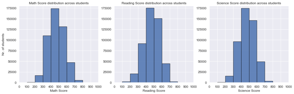
From the above distributions, we find out that:

• The literacy scores are spread out in a clear, smooth unimodal distribution of values
• The vast majority of the students are scoring in each subject between 300 and 600 points, while a small portion of the total number achieves poorer (between 100 and 300 points) or greater (between 600 and 800 points) test performance
• For each of these three score distributions, most students fitted within the interval of scores between 400 and 500 points, which happens to also be the middle interval of the possible score range. This shows that the PISA 2012 test has been constructed in a balanced manner with respect to student reviewing methodology and the difficulty of its questions

Visualisation 2

Next, we are interested in finding out about which countries host “exceptionally performing” students, and what their number is, with respect to each country and subject.

Since we have found out that a distribution of scores between 100 and 800 points is large enough to be noticed in our histogram of score count distributions, we understand that “exceptionally high” scores will be valued above 800 points.In [17]:

# Retrieve entries of students with scores above 800 points in each subject

high_math_score = df[df['Math Score'] > 800]['Country'].value_counts()
high_reading_score = df[df['Reading Score'] > 800]['Country'].value_counts()
high_science_score = df[df['Science Score'] > 800]['Country'].value_counts()

In [18]:

plt.figure(figsize = [15, 5])
plt.subplots_adjust(wspace = 0.6) # adjust spacing between subplots, in order to show long country names nicely
x_lim_max = high_math_score.values[0] + 6 # '+6' is done in order to show the text counts properly next to the bars


plt.subplot(1, 3, 1)
sb.barplot(y = high_math_score.index, x = high_math_score.values, color = sb.color_palette()[0])
plt.title('Students with Math score > 800');
plt.xlabel('Nr. of students')
plt.ylabel('Countries (ordered by student count)')

# Write the total number of students with exceptionally high scores in each country, right after the horizontal count bar
indexes, labels = plt.yticks()
for index, label in zip(indexes, labels):
    plt.text(y = index, x = high_math_score[label.get_text()] + 1, s = high_math_score[label.get_text()], va = 'center')
plt.xlim(0, x_lim_max);    


plt.subplot(1, 3, 2)
sb.barplot(y = high_reading_score.index, x = high_reading_score.values, color = sb.color_palette()[0])
plt.xlim(0, x_lim_max);
plt.title('Students with Reading score > 800');
plt.xlabel('Nr. of students')

# Write the total number of students with exceptionally high scores in each country, right after the horizontal count bar
indexes, labels = plt.yticks()
for index, label in zip(indexes, labels):
    plt.text(y = index, x = high_reading_score[label.get_text()] + 1, s = high_reading_score[label.get_text()], va = 'center')
plt.xlim(0, x_lim_max);    


plt.subplot(1, 3, 3)
sb.barplot(y = high_science_score.index, x = high_science_score.values, color = sb.color_palette()[0])
plt.xlim(0, x_lim_max);
plt.title('Students with Science score > 800');
plt.xlabel('Nr. of students')

# Write the total number of students with exceptionally high scores in each country, right after the horizontal count bar
indexes, labels = plt.yticks()
for index, label in zip(indexes, labels):
    plt.text(y = index, x = high_science_score[label.get_text()] + 1, s = high_science_score[label.get_text()], va = 'center')
plt.xlim(0, x_lim_max);

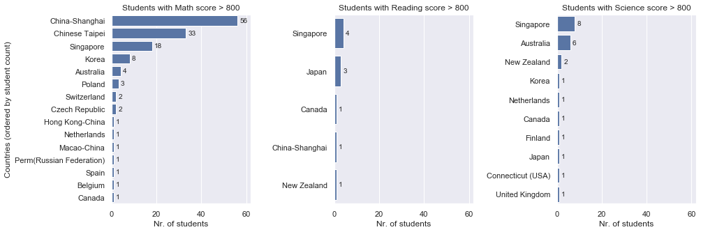
Here, we have counted the total number of exceptional students for each subject, and from their count distributions, we find out that:

• Oceania and Asian countries, in particular China and Singapore, seem to be the places where exceptional students are most likely to stem from
• Singapore is the clear leader in excellency, since it manages to reach within the top 3 countries with most exceptional students in all three areas of study
• Korea and Australia also have a respectable number of excellent students in both Math and Science
• Besides Asia and Oceania, a number of European and North American countries also make the podium: Canada is present in all three of the above distributions, while Poland, Czech Republic and Switzerland appear to be educating Math-bright students

Visualisation 3

Lastly, we would like to find out whether students with heterogenous family roots provide different score readings, on average, than students raised by parents with a homogenous family background.

For that, we would first like to see the proportion of students having parents with same or different cultural background:In [19]:

plt.figure(figsize=[3, 5]);
sb.countplot(x = 'Parents - Same Cultural Background', data = df, color = sb.color_palette()[0]);

y_ticks = np.arange(0, 450000 + 1, 50000)
plt.yticks(y_ticks, y_ticks);
plt.ylabel("Nr. of students");
plt.title('Family background distribution');

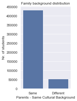
From this previous distribution, we discover that there are almost 9 times more students having parents with same cultural background than those having parents with different backgrounds.

Bivariate Exploration and Analysis

In this section, we will investigate the relationships between pairs of relevant variables in our data.

Visualisation 4

After finding out previously the global distribution of scores for each literacy category in part, we are interested to look into the relationship how the country of residence/education affects scores on each of the subjects individually.

Also, we have previously discovered countries where exceptional students stem from, such as China, Singapore, Korea or Poland.

Was this just a strong deviation from the norm of scores within these countries, or are these countries also between the top leaders when it comes to educating all of their students in these subjects?In [20]:

plt.figure(figsize = [15, 35])
plt.subplots_adjust(wspace = 0.85) # adjust spacing between subplots, in order to show long country names nicely

math_score_country_order = df.groupby('Country')['Math Score'].mean().sort_values(ascending = False).index
reading_score_country_order = df.groupby('Country')['Reading Score'].mean().sort_values(ascending = False).index
science_score_country_order = df.groupby('Country')['Science Score'].mean().sort_values(ascending = False).index

plt.subplot(1, 3, 1)
sb.boxplot(x = df['Math Score'], y = df['Country'], order = math_score_country_order, color = sb.color_palette()[9]);
plt.ylabel('Countries (ordered descendingly by score ranking)')
plt.title('Math score distributions by country');

plt.subplot(1, 3, 2)
sb.boxplot(x = df['Reading Score'], y = df['Country'], order = reading_score_country_order, color = sb.color_palette()[9]);
plt.ylabel(''); # Remove the redundant label
plt.title('Reading score distributions by country');

plt.subplot(1, 3, 3)
sb.boxplot(x = df['Science Score'], y = df['Country'], order = science_score_country_order, color = sb.color_palette()[9]);
plt.ylabel(''); # Remove the redundant label
plt.title('Science score distributions by country');

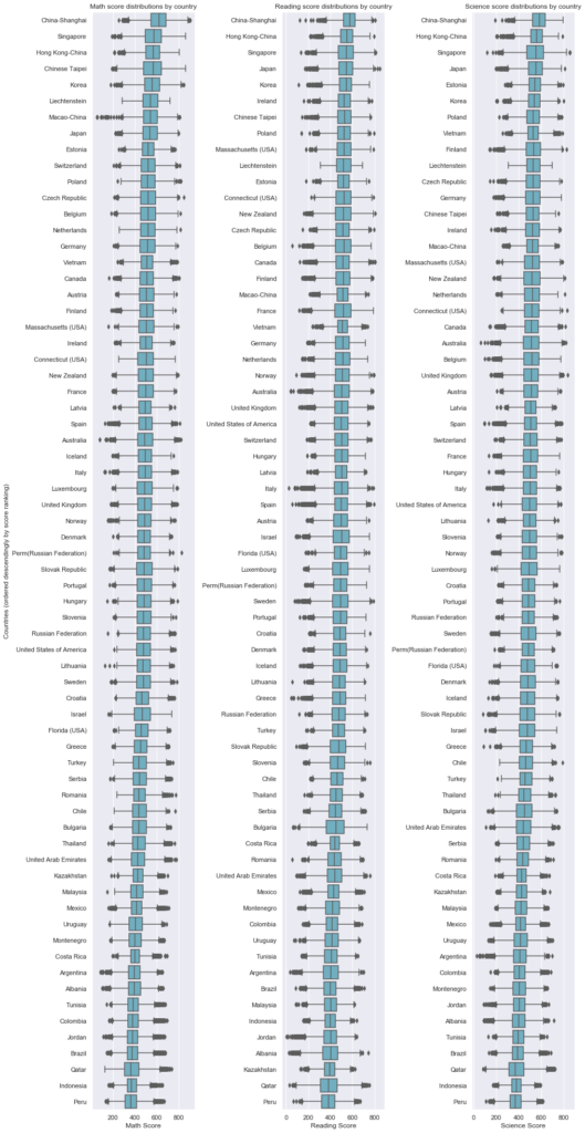
Here we have, in decreasing order, the rankings of countries with the best-performing students, on average, for each of the three subjects. We find that:

• Most countries seem to achieve, in different subjects, rankings which are close to each other, with 80% of countries reaching rankings within 10 places higher/lower across all the subjects. The remaining 20% of countries with large deviations will be analyzed further on, as we would like to find out in what subjects are they deviating and how large is the difference
• From the top ranking of countries, we can clearly see that it was no coincidence that exceptional students come from Asian countries, in particular China and Singapore, as these are the countries which are 1st, 2nd or 3rd place across all subjects. Another country which impressed was Poland, with 3 exceptional students in Mathematics. Here, it can be seen that this is no coincidence either, as Poland occupies a spot in the top 10 placements in Reading and Science, and 11th in Mathematics
• The box-and-wiskers plot allows us to see the outliers in scores for each country in part. For example, we find out that, even though a number of Singapore’s students managed to achieve outstanding results in the field of Mathematics, that is not to be considered “out of ordinary” (or, with other words, as outliers) in the country’s perspective, however the outstanding results received in Science can be indeed considered to be slightly out of regular bounds, since we can notice the Singapore’s outliers in the plot
• Other such findings can be performed by picking a country of interest and checking its score distribution, rankings and outlier distribution accordingly

Visualisation 5

Further on, we are interested to see if there are any countries which had multi-talented students, performing exceptionally (score > 800) in not only one discipline, but in multiple ones at the same time.

In [21]:

high_math_and_reading_score = df[(df['Math Score'] >= 800) & (df['Reading Score'] >= 800)]['Country'].value_counts()
high_math_and_science_score = df[(df['Math Score'] >= 800) & (df['Science Score'] >= 800)]['Country'].value_counts()
high_reading_and_science_score = df[(df['Reading Score'] >= 800) & (df['Science Score'] >= 800)]['Country'].value_counts()

In [22]:

plt.figure(figsize = [15, 1])
plt.subplots_adjust(wspace = 0.6) # adjust spacing between subplots, in order to show long country names nicely
x_lim_max = high_math_and_science_score.values[0] # adjust the proportions of the x-axis with respect to all 3 plots using this

plt.subplot(1, 3, 1)
sb.barplot(y = high_math_and_reading_score.index, x = high_math_and_reading_score.values, color = sb.color_palette()[0])
plt.title('Students with Math & Reading scores > 800');
plt.xticks(np.arange(0, x_lim_max + 2, 1));

plt.subplot(1, 3, 2)
sb.barplot(y = high_math_and_science_score.index, x = high_math_and_science_score.values, color = sb.color_palette()[0])
plt.title('Students with Math & Science scores > 800');
plt.xticks(np.arange(0, x_lim_max + 2, 1));

plt.subplot(1, 3, 3)
sb.barplot(y = high_reading_and_science_score.index, x = high_reading_and_science_score.values, color = sb.color_palette()[0])
plt.title('Students with Reading & Science scores > 800');
plt.xticks(np.arange(0, x_lim_max + 2, 1));

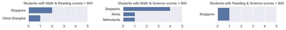
We have once again realized plots to visualize the distribution of counted students with exceptional results in multiple fields. It can be found that:

• Singapore leads in the world ranking of multi-talented outstanding results, being the only one country present in all three possible combination of two talents. Coupled together with previous findings of Singapore’s on-average and above-average student results, we can determine that its country is world-leader in providing multidisciplinary high-quality education, across all measured disciplines.
• China is once again present in the rankings, together with (South) Korea, determining that, as said about Singapore, such countries have a very high quality of education in the measured fields. The connection between all previous visualizations of scores determine that such outstanding results are not simple coincidence, but only slightly-higher than average results compared with these countries’ mean of scores.
• There were no students who have managed to reach scores above 800 in all three subjects simultaneously, which is why there is no further visualization on this matter.

Visualisation 6

Lastly, we are investigating whether students having parents from different cultural (country) backgrounds are performing differently than students whose parents come from the same type of background.In [23]:

plt.figure(figsize = [15, 4])
plt.subplots_adjust(wspace = 1.2)

plt.subplot(1, 3, 1)
sb.boxplot(x = df['Parents - Same Cultural Background'], y = df['Math Score'], palette = 'Set2')
plt.title('Math scores related to family background');

plt.subplot(1, 3, 2)
sb.boxplot(x = df['Parents - Same Cultural Background'], y = df['Reading Score'], palette = 'Set2')
plt.title('Reading scores related to family background');

plt.subplot(1, 3, 3)
sb.boxplot(x = df['Parents - Same Cultural Background'], y = df['Science Score'], palette = 'Set2');
plt.title('Science scores related to family background');

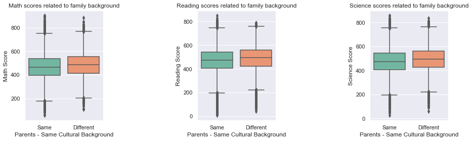
It can be seen that, on average, indeed students coming from heterogenic family backgrounds report increased performance in all areas, compared to students from homogenous family backgrounds.

Multivariate Exploration and Analysis

In this section, we will investigate the relationships between the interactions of three or more variables at the same time.

Visualisation 7

Out of curiosity, we would like to know whether it is normal that most countries who had many students scoring high in one of the subjects, also had, on average, students scoring high on the other two subjects.

Therefore, we are going to study the pair-by-pair relationship between Math Scores, Reading Scores and Science Scores, and correlate them in pair scatter plots, in order to see what type and strength of correlation exists.In [24]:

grid = sb.pairplot(data = df, vars=["Math Score", "Reading Score", "Science Score"]);
grid.fig.suptitle("Pair-by-pair representation of different scores' correlation", y = 1.02);

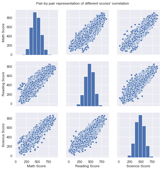
As it could be expected, there is a very strong and positive correlation between any pair of the three variables representing the scores of the three subjects. Therefore, the previous relationships between scores observed in the behaviour of many countries’ students is justified.

Visualisation 8

Lastly in this analysis, even though we found out that positive correlation of students’ scores is normal behaviour for a country, and that most countries display similar rankings in scores across all three subjects, there are still 20% of countries who deviate from this behaviour, where these countries have differences in rankings of some scores of more than 10 places.

We will look into who are those countries, and where do the differences take place in the scores of each of these countries.

In [25]:

country_outliers = []

for country in df['Country'].unique():
    if ((np.abs((math_score_country_order.get_loc(country) - reading_score_country_order.get_loc(country))) > 10) |\
        (np.abs((math_score_country_order.get_loc(country) - science_score_country_order.get_loc(country))) > 10) |\
        (np.abs((reading_score_country_order.get_loc(country) - science_score_country_order.get_loc(country))) > 10)):
        
        country_outliers.append(country)
        
        
country_outliers.sort() # Sort countries alphabetically

for country in country_outliers:
    print((country) + ':' + str((len('United States of America:') - len(country) + 1) * ' ') + 'Math place: ' + str(math_score_country_order.get_loc(country)) + str((5 - len(str(math_score_country_order.get_loc(country))) + 1) * ' ') + 'Reading place: ' + str(reading_score_country_order.get_loc(country)) + str((5 - len(str(reading_score_country_order.get_loc(country))) + 1) * ' ') + 'Science place: ' + str(science_score_country_order.get_loc(country)))

Austria:                   Math place: 17    Reading place: 31    Science place: 23
Florida (USA):             Math place: 44    Reading place: 33    Science place: 40
Iceland:                   Math place: 27    Reading place: 40    Science place: 42
Ireland:                   Math place: 20    Reading place: 5     Science place: 13
Israel:                    Math place: 43    Reading place: 32    Science place: 44
Kazakhstan:                Math place: 53    Reading place: 65    Science place: 54
Macao-China:               Math place: 6     Reading place: 17    Science place: 14
Massachusetts (USA):       Math place: 19    Reading place: 8     Science place: 15
Norway:                    Math place: 31    Reading place: 22    Science place: 33
Slovak Republic:           Math place: 34    Reading place: 45    Science place: 43
Slovenia:                  Math place: 37    Reading place: 46    Science place: 32
Switzerland:               Math place: 9     Reading place: 26    Science place: 26
United States of America:  Math place: 39    Reading place: 25    Science place: 30
Vietnam:                   Math place: 15    Reading place: 19    Science place: 7

In [26]:

df_country_outliers = df[['Country', 'Math Score', 'Reading Score', 'Science Score']][df['Country'].isin(country_outliers)]
df_country_outliers = df_country_outliers.melt('Country', var_name = 'Score Type', value_name = 'Scores')

In [27]:

plt.figure(figsize = [7, 10])

sb.pointplot(x = 'Scores', y = 'Country', hue = 'Score Type', data = df_country_outliers, linestyles = '', dodge = 0.4, ci = 'sd', palette = 'deep', order = country_outliers);
plt.legend(loc = 2);
plt.title('Score distribution across subjects of countries with strong deviations in results');

From this visualization, we can better understand the deviations in the outlier-countries’ score pattern. For example, we find out that Kazakhstan is deviating due to much weaker scores in Reading than in the other two disciplines; while Switzerland is deviating through much higher scores in Mathematics than in the other two subjects. For any country of interest, such an analysis can be performed.

Conclusions and Answers

Lastly, we will restate our three questions of interest, along with a summary of our conclusions:

• How do students from individual countries perform in Math, Reading and Science literacy?
  • We have found the literacy trends for each country in part, along with countries with high deviations in scores compared to the norm. The results can be explored in Visualization 4 and 8.

• What are the countries from which “geniuses” stem, meaning which countries have students with exceptionally high literacy scores?
  • Generally, we have seen Asian countries as being the world leaders at educating students who perform exceptionally, not only in each different subject individually, but also at multiple subjects simultaneously. Singapore and China are examples of this.

• Do students whose parents have different cultural backgrounds report any changes in average scores, compared with students raised in a homogeneous family background?
  • We have discovered that students whose parents are from two different cultural backgrounds report, on average, slightly higher performance (scores) in all three measured subjects.